Learning Strategies for Patch-Based Local Descriptors

Some computer vision tasks — camera localization, 3D reconstruction — depend on geometric relationships between images. One way to recover these relationships is through matching local features. Local features are extracted from small local regions of an image: edges, corners, lines, curves, and distinctive regions. A local feature generally has two components: the keypoint location, and a descriptor. Descriptors can be handcrafted or learned.

This post focuses on the learned case: given known keypoints, how do you train a network to generate descriptors for local patches? Rather than architectural details, the focus is on how different papers approach data processing and learning strategy.

Data and task

The basic task is: given a patch, produce a descriptor. The network takes a local image patch as input and outputs a feature vector.

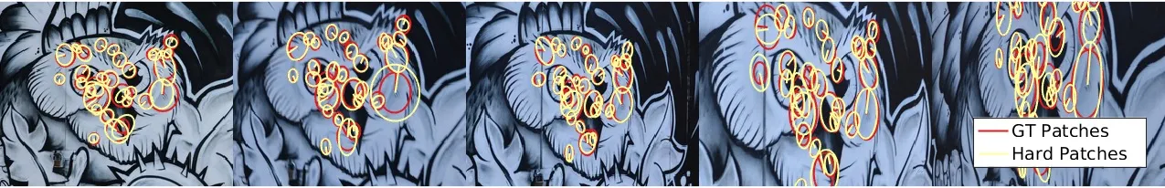
Patches are extracted around keypoints in the image. In the figure below, five images come from the same scene. The center of each circle is a keypoint; the circled region is the extracted patch.

{%asset_img images_hard.jpg HPatch images and keypoints %}

Since all five images share the same scene, keypoints correspond across images. In the figure below, each column shows patches from matching keypoints; each row shows all patches extracted from one image.

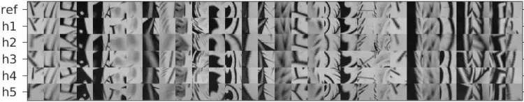
{%asset_img patches_hard.jpg HPatch extracted local patches %}

An ideal descriptor makes matched keypoints close in descriptor space and unmatched keypoints far apart. Applied to the figure above: patches in the same column should have similar descriptors; patches in the same row should be far from each other.

Formally: let keypoint have descriptor — called the anchor. A matching keypoint has descriptor (positive sample). A non-matching keypoint has descriptor (negative sample). The goal is .

Training pipeline

A common training pipeline for patch-based local descriptors:

{%asset_img general_pipeline.jpg Pipeline %}

Data sampling

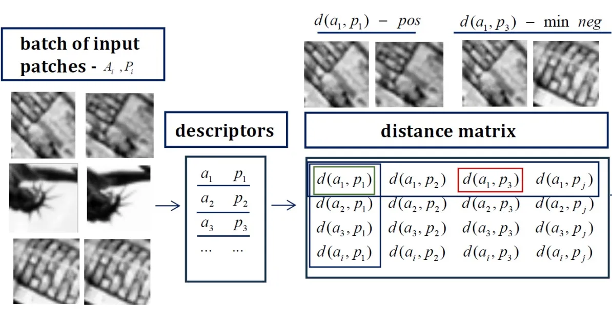
Randomly sample matching patch pairs to form each training batch: , where is a matched pair.

Descriptor and distance matrix

The network produces descriptors for each pair . Computing pairwise distances between all anchors and positives in the batch gives the distance matrix shown on the right side of the figure. Distances between matched pairs are positive-pair distances; distances between unmatched pairs are negative-pair distances.

Different loss functions can then be applied to this descriptor/distance matrix.

Learning strategies

L2Net | L2-Net: Deep Learning of Discriminative Patch Descriptor in Euclidean Space

L2Net is an early deep learning-based patch descriptor. Its loss function is largely out of use today, but the model architecture remains widely referenced.

The L2Net loss has three terms:

Descriptor similarity: uses relative distances to separate matching from non-matching patch pairs — softmax over rows and columns of the distance matrix.
Descriptor compactness: penalizes correlation among dimensions of the output feature vector, pushing the descriptor toward a more compact representation.
Intermediate feature maps: applies additional supervision to intermediate feature maps during training, improving final performance by taking the distance matrix at each intermediate layer and computing softmax over its rows and columns.

The L2Net architecture:

flowchart LR
    Input[Patch] --> B(3x3 Conv 32):::Conv
    B --> C(3x3 Conv 32):::Conv
    C --> D(3x3 Conv 64/2):::ConvDown
    D --> E(3x3 Conv 64):::Conv
    E --> F(3x3 Conv 128/2):::ConvDown
    F --> G(3x3 Conv 128):::Conv
    G --> H(8x8 Conv 128):::ConvBN
    H --> J(LRN):::LRN
    J --> Descriptor(Descriptor)

    classDef Conv fill:#cfc;
    classDef ConvDown fill:#cff;
    classDef ConvBN fill:#ffc;
    classDef LRN fill:#fcc;

3×3 Conv means Conv+BN+ReLU; 8×8 Conv means Conv+BN. Layers 3 and 5 use stride 2 for downsampling. LRN (Local Response Normalization) normalizes the output, equivalent to L2Norm. In practice, an InstanceNorm layer is commonly added at the beginning to reduce the effect of lighting and other appearance variations.

The network is simple and fast — feature extraction runs in the millisecond range, typically around 1ms on a modest GPU.

HardNet | Working hard to know your neighbor’s margins: Local descriptor learning loss

{%asset_img hardnet_pipeline.jpg HardNet_Pipeline %}

HardNet uses metric learning’s triplet loss to maximize the margin between positive and negative pairs within each training batch.

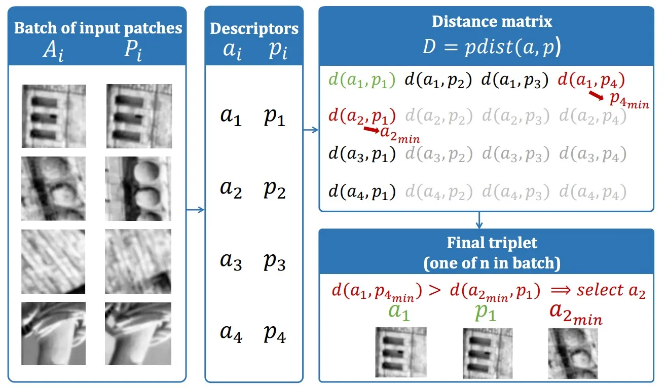
Given the distance matrix, for each matched pair the following can be identified:

: anchor descriptor
: positive descriptor
: the non-matching descriptor closest to , where — corresponds to in the figure
: the non-matching descriptor closest to , where — corresponds to in the figure

Each matched pair generates a tuple with distances:

: anchor-positive distance
: anchor-negative distance
: anchor-negative distance

Training on the hardest negatives (smallest anchor-negative distances) maximizes the margin. The loss is:

Implementation:

def triplet_loss(x, label, margin=0.1):
    # x is D x N
    dim = x.size(0) # D
    nq = torch.sum(label.data==-1).item() # number of tuples
    S = x.size(1) // nq # number of images per tuple including query: 1+1+n

    xa = x[:, label.data==-1].permute(1,0).repeat(1,S-2).view((S-2)*nq,dim).permute(1,0)
    xp = x[:, label.data==1].permute(1,0).repeat(1,S-2).view((S-2)*nq,dim).permute(1,0)
    xn = x[:, label.data==0]

    dist_pos = torch.sum(torch.pow(xa - xp, 2), dim=0)
    dist_neg = torch.sum(torch.pow(xa - xn, 2), dim=0)

    return torch.sum(torch.clamp(dist_pos - dist_neg + margin, min=0)) / nq

SOSNet | SOSNet: Second Order Similarity Regularization for Local Descriptor Learning

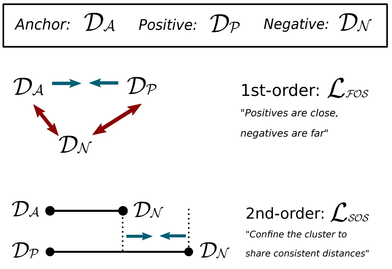
HardNet’s loss is based on first-order distances. SOSNet adds a second-order similarity term on top of it.

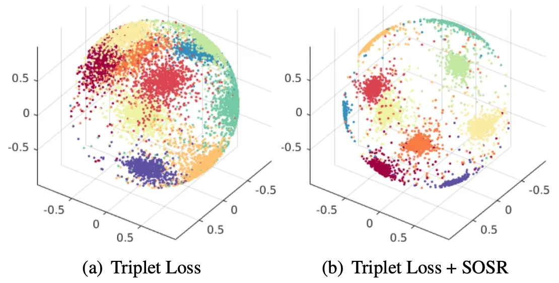
Second-order distance here refers to the distance between the two anchor-negative distances within a tuple : . Minimizing this second-order distance pulls descriptors into tighter clusters, as shown below.

{%asset_img second_order_dist.jpg Second_Order_Distance %}

{%asset_img sosnet.jpg SOSNet_output %}

Implementation:

def sos_loss(x, label):
    # x is D x N
    dim = x.size(0) # D
    nq = torch.sum(label.data==-1).item() # number of tuples
    S = x.size(1) // nq # number of images per tuple including query: 1+1+n

    xa = x[:, label.data==-1].permute(1,0).repeat(1,S-2).view((S-2)*nq,dim).permute(1,0) # D * (B * num_neg)
    xp = x[:, label.data==1].permute(1,0).repeat(1,S-2).view((S-2)*nq,dim).permute(1,0)
    xn = x[:, label.data==0]

    dist_an = torch.sum(torch.pow(xa - xn, 2), dim=0)
    dist_pn = torch.sum(torch.pow(xp - xn, 2), dim=0)

    return torch.sum(torch.pow(dist_an - dist_pn, 2)) ** 0.5 / nq

Log Polar Transformation | Beyond Cartesian Representations for Local Descriptors

Another useful contribution for local feature learning is log-polar transformation. The core idea is to transform the image from Euclidean coordinates to log-polar coordinates as a preprocessing step. Rotation and scale changes have little effect on images in log-polar coordinates, which gives the model better robustness to these transformations.

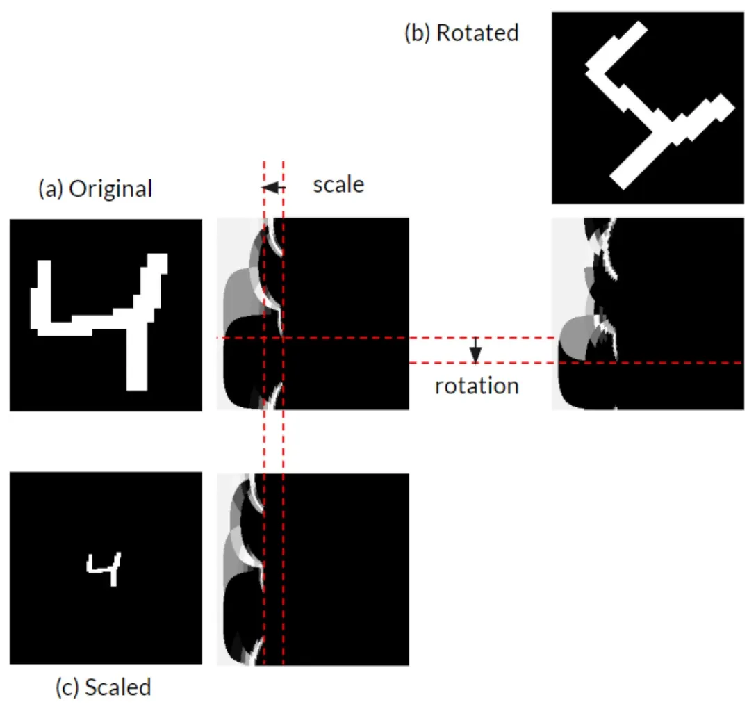
{%asset_img log_polar_transformation.jpg Rotation and Scaling transformations to a Euclidean image can be read as horizontal and vertical shift respectively, after a log-polar transformation. The log-polar transformation translates rotation and scale in Euclidean images into vertical and horizontal translations (respectively) in the log-polar model. %}

As shown above, rotation and scale changes in Euclidean images correspond to vertical and horizontal translations in log-polar space. Convolution’s sliding window operation is inherently robust to translation, which is why this helps. Note that typical patch-based CNNs are quite shallow and can’t easily cancel the bias introduced by rotation and scale variation — in practice, the gravity direction is often used to pre-rotate patches before feeding them to the CNN. Log-polar transformation sidesteps this by building the invariance into the preprocessing.

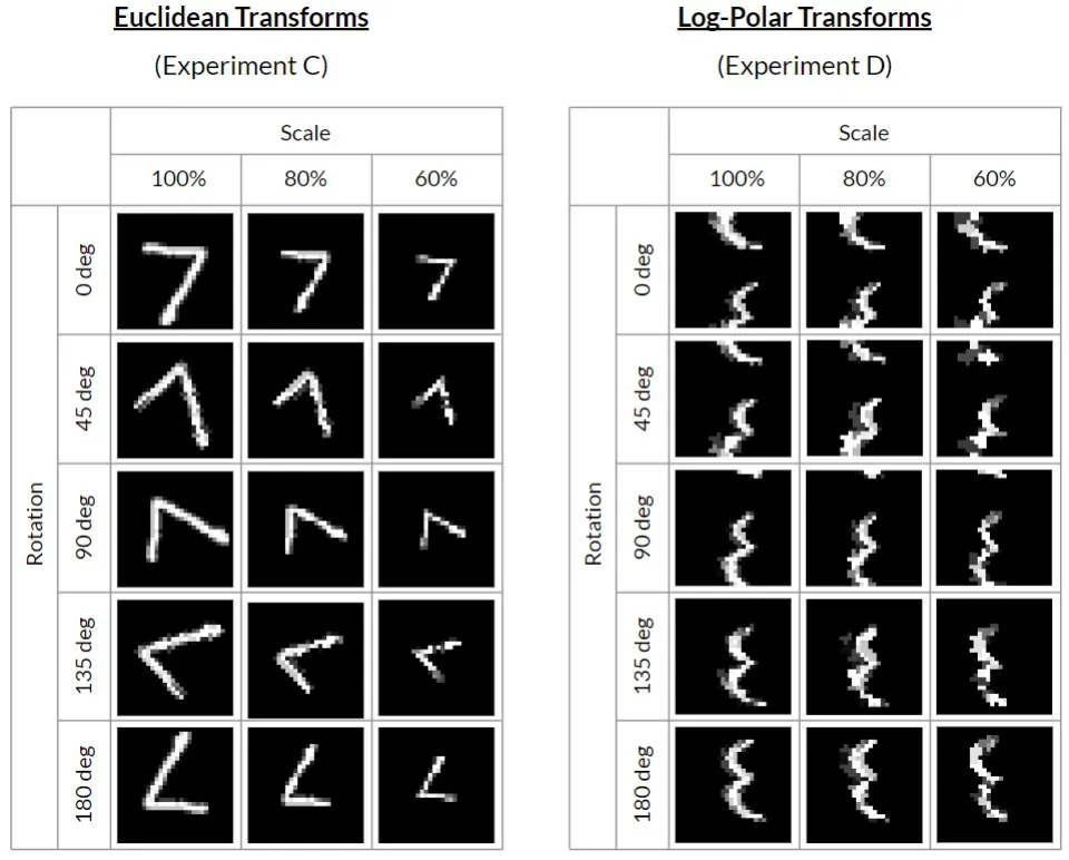
More examples of how rotation and scale transformations appear in both coordinate systems:

{%asset_img log_poloar_samples.jpg Example of rotation and scale transformations for a single MNIST image. %}

Log-polar transformation as a preprocessing step:

def to_log_polar(img, dsize, max_radius):
    assert isinstance(img, Image.Image)

    # dsize = img.size
    center = [s // 2 for s in img.size]
    flags = cv2.WARP_POLAR_LOG
    out = cv2.warpPolar(
        np.asarray(img), dsize=dsize, center=center, maxRadius=max_radius, flags=flags
    )
    return Image.fromarray(out)


def from_log_polar(polar_img, dsize, max_radius):
    assert isinstance(polar_img, Image.Image)

    # dsize = polar_img.size
    center = [s // 2 for s in polar_img.size]
    flags = cv2.WARP_POLAR_LOG | cv2.WARP_INVERSE_MAP
    out = cv2.warpPolar(
        np.asarray(polar_img),
        dsize=dsize,
        center=center,
        maxRadius=max_radius,
        flags=flags,
    )
    return Image.fromarray(out)

Note that because PyTorch’s GridSample uses a different convention, the OpenCV-based log-polar transform won’t match the output of the paper’s original PTN network. For the original PTN implementation, see the paper’s code.