When benchmarking deep learning inference, people reach for FLOPs and parameter count as proxies for model size. The problem is that swapping Conv for DepthWise Conv to cut FLOPs often fails to speed up the deployed model in any meaningful way.
This post covers four metrics for model size — FLOPs, parameter count, MACs (memory access cost), and memory footprint — looks at how each affects inference performance, and wraps up with network design recommendations for different hardware. It is reprinted from Zichen Tian’s Zhihu column.
Common model size metrics
FLOPs
FLOPs are the most widely used model size metric, and many papers compare baselines on this basis.
FLOPs (Floating Point Operations) count the total arithmetic operations the model requires. Float32 is the most common data format, so FLOPs is standard — I’ll use it throughout.
Total FLOPs is the sum across all operators. For Eltwise Sum of two
PyTorch has several FLOPs counting tools, but they can miss certain operators and count them as zero. The discrepancy is usually small.
Parameter count
Early papers used parameter count as the main model size metric.
Parameter count is the total number of trainable parameters, which determines disk footprint. For CNNs, Conv and FC weights dominate; other operators contribute negligible parameters.
Parameter count feeds into MACs (it’s part of what the hardware reads), so it doesn’t directly drive inference speed. It does affect memory footprint and startup time.
It also determines package size — a real constraint for mobile apps with strict APK limits, and for embedded devices with limited flash. Beyond trimming parameters at design time, model compression helps. Protobuf (Caffe and ONNX) encodes compactly, at the cost of decompression overhead at startup.
Memory access volume (MACs)
MACs are the most commonly overlooked metric, and probably the one with the most impact on inference performance in modern hardware.
MACs (Memory Access Cost) count the total bytes read and written during inference. For Eltwise Sum of two
MACs have a large effect on inference speed and are worth tracking whenever you’re designing a model.
Memory footprint
Memory footprint is how much RAM or VRAM the model uses at runtime. Peak usage is what usually matters; average is sometimes tracked. Memory footprint is not the same as MACs.
It rarely appears in papers because it depends on software as much as architecture. Some frameworks pre-allocate everything upfront (footprint = sum of all tensors). Most also offer a “lite” mode with dynamic allocation, which cuts peak usage at a small performance cost.
Like parameter count, memory footprint doesn’t directly drive inference speed. But on systems with concurrent tasks — inference servers, automotive platforms, mobile apps — predictable usage matters. Too much, and other tasks can’t run. Unpredictable spikes cause their own problems.
Summary
FLOPs, parameter count, MACs, and memory footprint each measure model size from a different angle. The right metric depends on what you’re optimizing for.
Inference speed is not just about FLOPs. MACs often matter more. The next section gets into why.
Does fewer FLOPs mean faster inference?
No.
There’s no direct causal relationship between FLOPs and inference latency. FLOPs are a reference, not a predictor.
Inference speed on given hardware depends on FLOPs, MACs, hardware characteristics, software implementation, system environment, and more. When you have the hardware and can test quickly, measure directly — that’s always the most accurate estimate.
When designing networks, if you can run quick benchmarks, start testing performance early in the iteration cycle. Some NAS approaches fold latency measurement into the search itself, or model the hardware as a direct parameter. Networks designed this way need far less performance work at deployment time.
I’ll cover computational intensity and the RoofLine model, compute-bound vs. memory-bound operators, and inference time.
Computational intensity and the RoofLine model
Computational intensity
The RoofLine model gives the performance ceiling a program can reach on given hardware:
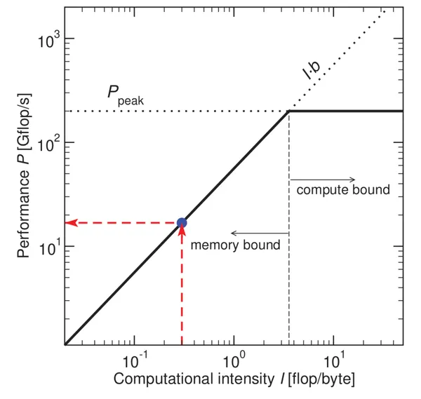
When
When
At the intersection, both compute and bandwidth peak simultaneously.
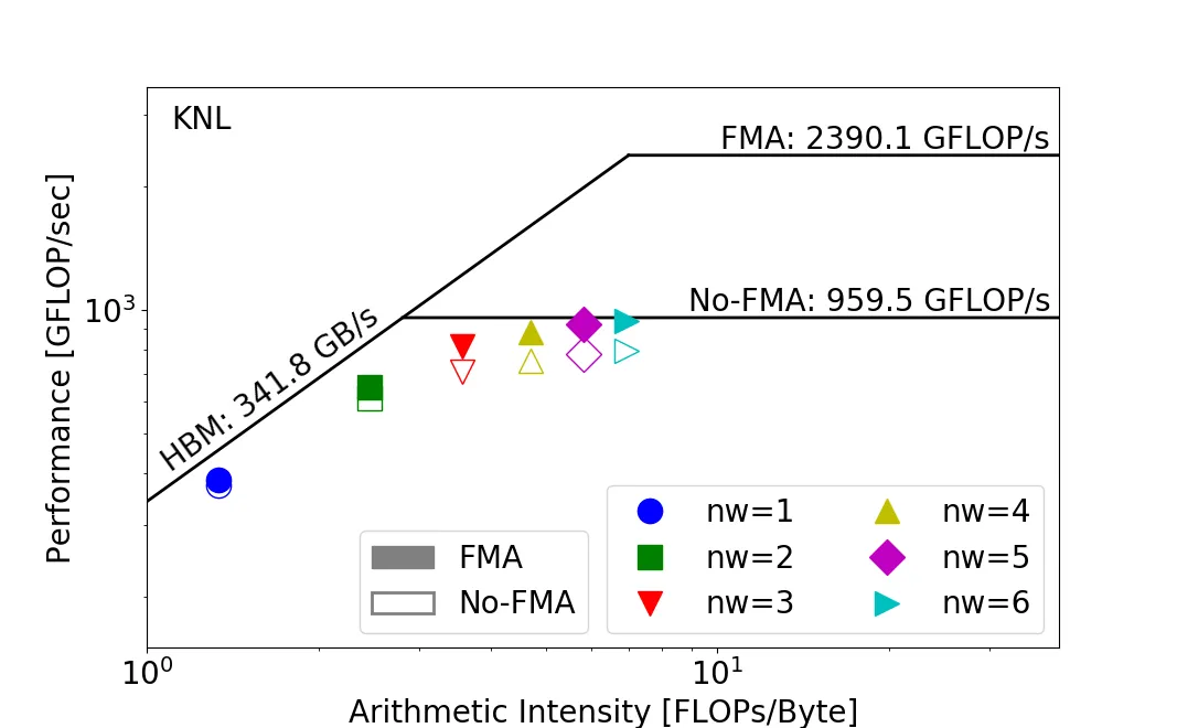
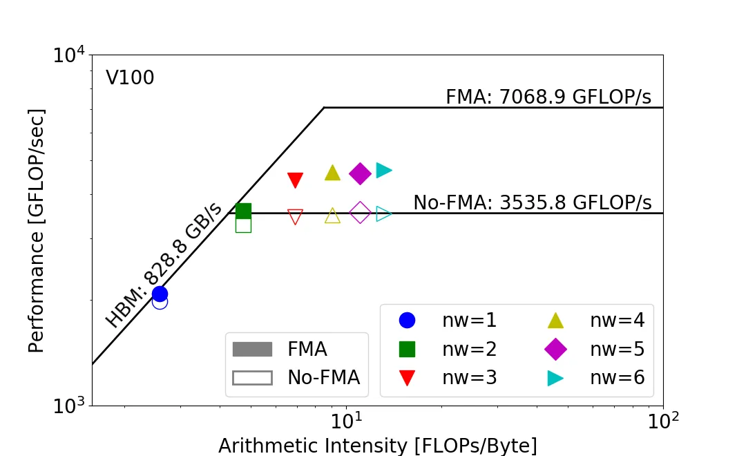
The same program can land in different regions on different hardware. A program that’s memory-bound on Intel KNL can be compute-bound on NVIDIA V100. To fully use the KNL, you’d want to push its computational intensity higher.
Compute-bound vs. memory-bound operators
Operators split by computational intensity. Conv, FC, and Deconv are generally compute-bound; ReLU, Eltwise Add, and Concat are memory-bound.
The same operator can switch categories based on its parameters. Increasing Conv group count, or reducing input channels, drops intensity — sometimes enough to flip it from compute-bound to memory-bound.

The spread across convolution configurations is large. Depthwise Conv has an intensity of just 2.346, which makes it memory-bound on most modern hardware.
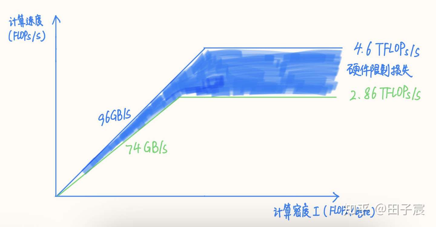
Higher intensity generally means better hardware utilization. On an Intel 10980 XE at 16 cores and 4.5 GHz: theoretical FP32 throughput is 4.608 TFLOPs/s, theoretical bandwidth is 96 GB/s. The ridge point sits at intensity 48.
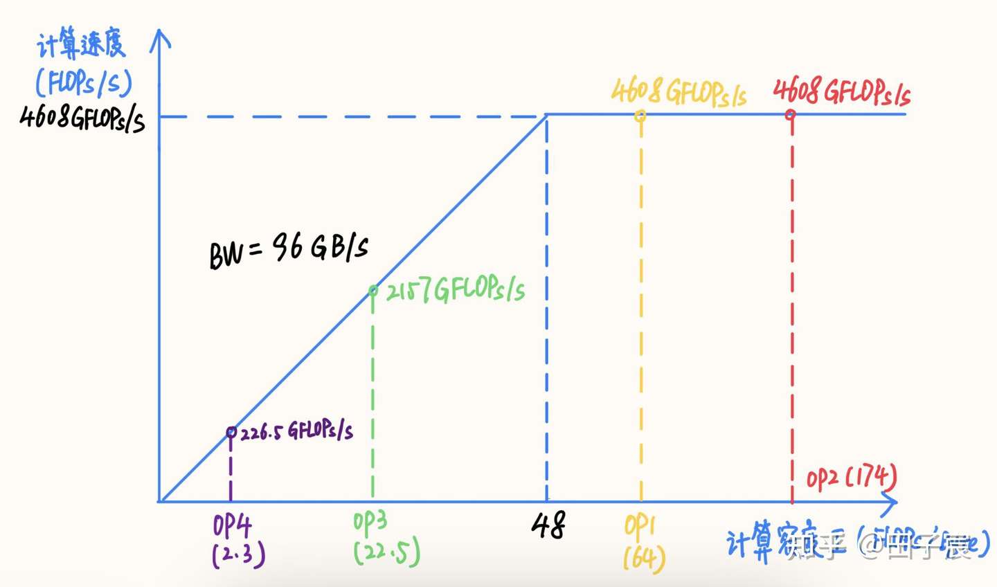
OP1 and OP2 are compute-bound and reach peak throughput. OP3 and OP4 are memory-bound and can’t — OP4, with its tiny intensity, hits only 4.9% compute efficiency.
Inference time
There’s a persistent vocabulary mismatch between deployment engineers and algorithm engineers. Deployment folks talk about “compute efficiency”; algorithm folks care about “inference time.” These are not the same, and the confusion causes real problems in handoffs.
Inference time follows directly from the RoofLine model:
Breaking it into cases:
Memory-bound operators: inference time scales with MACs. Compute-bound operators: it scales with FLOPs.
In the compute-bound region, fewer FLOPs means less latency. In the memory-bound region, FLOPs are irrelevant; latency tracks MACs. Globally, FLOPs and inference time are not linear.
OP4 was terrible on compute efficiency, but it also had very low MACs, so it was actually faster than the others. Its FLOPs were 1/130 of OP1’s, but latency only fell to 1/6. That’s exactly why I once cut a model to 1/10 the FLOPs and saw almost no speedup.
Consider two more examples. These two convolutions have similar FLOPs but both are memory-bound. OP3 has far lower MACs than OP5, so it runs faster:

And OP5 vs. OP6: one is depthwise Conv, the other is standard Conv, everything else identical. You’d expect depthwise to be faster. Their inference times are essentially the same:

Summary
FLOPs alone can’t predict inference latency. Different platforms have different ridge points — compute-bound on Intel X86 (ridge at intensity 48) may be memory-bound on NVIDIA V100 (ridge at 173.6). Same model, different behavior.
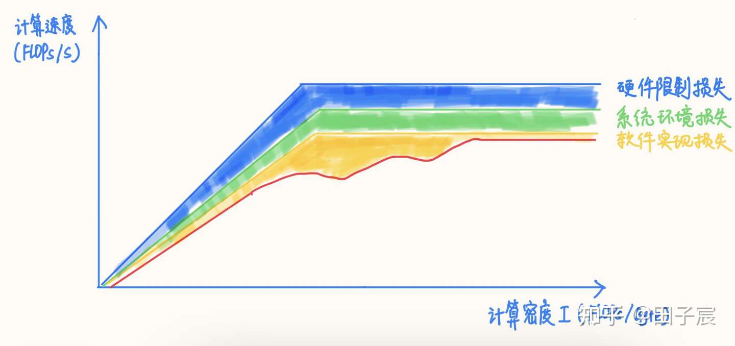
RoofLine is inherently nonlinear, so there are no universal conclusions. Hardware microarchitecture, system environment, and software implementation all chip away at the ceiling. The model gives an upper bound. Direct measurement gives the actual number.
What RoofLine is good for is reasoning: compute-bound programs are limited by throughput, memory-bound programs are limited by bandwidth. Keep that in mind when designing networks and you’ll stop wondering why cutting FLOPs in half didn’t make anything faster.
Other factors affecting inference performance
Hardware constraints
Spec-sheet peak throughput and bandwidth are theoretical. Real hardware usually falls short. Run micro-benchmarks first.
On the Intel X86 example: theoretical avx512 throughput assumes 4.5 GHz. Running avx512 across 16 cores, the CPU throttles to about 2.9 GHz — theoretical throughput drops to 2.96 TFLOPs/s, measured is 2.86 TFLOPs/s.
Some chips can’t reach theoretical peaks for other reasons: no multiple issue, no out-of-order execution, blocking cache design, or outright performance bugs. Memory has the same gap. This platform’s theoretical bandwidth is 96 GB/s; measured peak read bandwidth was 74 GB/s, about 77%.
With corrected numbers, the ridge point shifts, which can change operator classifications. Two useful tools:
System environment
Unless the program runs on bare metal, the OS adds overhead: scheduling, memory management, its own resource use.
For most deep learning inference, the OS impact is small. Two cases where it isn’t:
Android big.LITTLE scheduling: if a process doesn’t sustain high CPU utilization (periodic tasks are a common culprit), Android may migrate it to efficiency cores.
Linux page faults: when a process requests memory, the kernel returns a virtual page. The physical page isn’t allocated until the process actually touches it — triggering a kernel trap. At scale, this seriously hurts performance.
Both are fixable. CPU affinity binding handles the scheduling problem; physical page locking (requires kernel mode) or memory pooling handles page faults.
Other processes compete for the same resources. A model that passes performance testing in isolation can fail in production. Test in an environment that matches production as closely as possible.
Software implementation
Implementation quality has a large effect. Python nested loops vs. NumPy on the same matrix operation can differ by one to two orders of magnitude.
For inference frameworks, quality shows up in pipeline utilization, cache efficiency, algorithm complexity, OS issue handling, and graph optimization. So many things interact that performance effects are highly nonlinear — you can’t usually generalize, you measure.
Vector arithmetic and transcendental functions have similar FLOPs counts, but transcendental functions are typically slower because most hardware lacks SIMD support for them. Dilated Conv underperforms standard Conv because its memory access pattern is less cache-friendly.
Some rough guidelines:
- Memory-bound operators with sequential access patterns — Concat, Eltwise Sum, ReLU, LeakyReLU, ReflectionPad — approach measured bandwidth on large tensors. With graph fusion, the overhead is basically nothing.
- Compute-bound operators (Conv, FC, Deconv) at high intensity: most frameworks get close to peak throughput. At lower intensity, performance varies by framework. Higher intensity correlates with better utilization.
- Stick to common operator configs. Conv 3x3_s1/s2 and 1x1_s1/s2 get special-cased in most frameworks.
Summary
RoofLine gives you the ceiling. Hardware limits, OS overhead, and implementation quality all eat into it, often significantly and nonlinearly. Treat the analysis here as a thinking framework. Measure.
Network design recommendations for inference speed
Hardware, environment, and framework differences mean these recommendations won’t apply universally. When something doesn’t add up, talk to your deployment engineers.
Methodology:
- Get measured peak throughput and bandwidth for your target hardware. Spec sheets are starting points.
- Know the gap between test environment and production. Close it, or account for it.
- Match the network’s computational intensity to the platform’s ridge point.
- Track MACs and platform latency alongside FLOPs.
- Measure throughout the design iteration. Don’t wait until deployment to benchmark.
- Layer-by-layer profiling, done close to deployment engineers, is how you find and fix performance problems.
Network architecture:
- On low-throughput platforms (CPUs, budget GPUs), cutting FLOPs cuts latency directly.
- On high-throughput platforms (GPUs, DSPs), just cutting FLOPs doesn’t work. Watch MACs. Carelessly cutting FLOPs often pushes the network into the memory-bound region, where latency tracks MACs instead — and these platforms have weaker bandwidth relative to compute. A higher-intensity network can actually be faster than a lower-intensity one.
- Use standard architectures. Frameworks apply graph fusion to canonical patterns. Conv-BN-ReLU fuses into one operator; Conv-ReLU-BN doesn’t let the BN fuse.
- Standard configs: Conv 3x3_s1/s2, 1x1_s1/s2. These get optimized. Unusual configs don’t.
- Channel counts at multiples of 4/8/16/32. Most frameworks use data layouts that work best at these sizes.
- Framework overhead for topology management, memory pools, and thread pools scales with layer count. “Small and deep” networks pay more overhead than “large and shallow” ones. Usually negligible, but with many fragmented operators it can limit multi-thread scaling.
Other:
- Overlap inference with data loading. Hiding I/O latency costs nothing.
Algorithm engineers who understand this performance model can reason about deployment trade-offs themselves, rather than discovering at the end that their supposedly faster model didn’t actually get faster.
Are there model architectures with low MACs?
Some work, like ShuffleNetV2, has considered MACs in the design process. Nothing as canonical as DepthWise Conv exists for reducing MACs specifically.
My read on it:
- MACs can be reduced, but maintaining accuracy at the same time is hard. It takes dedicated research.
- Some ops reduce MACs for free — use them. Others inflate MACs needlessly — don’t.
- Quantization often saves more in bandwidth than in compute. When bandwidth is the bottleneck, that’s the more important win.
DWConv 3×3 + Conv 1×1 became canonical because both FLOPs decrease and accuracy holds. FLOPs you can compute before training. Accuracy you only know after. That asymmetry is part of why finding this structure took so much iteration.
ShuffleNetV2 uses MACs to pick group counts, but the overall block isn’t MACs-first. I haven’t followed the literature recently enough to know if there’s dedicated MACs-reduction work now (leave a comment if there is).
This feels like a productive research direction. Manual architecture search with MACs as the objective, or adding MACs to NAS, both seem viable. The manual approach has better interpretability; NAS might be easier to execute. One thing to keep in mind either way: reducing MACs only matters if your model is actually memory-bound on the target device. Compute-bound? Reducing MACs does nothing.
Deployment tips for not wasting MACs:
- Channel counts: multiples of 4/8/16/32. Frameworks pad channels for computation, so channel=23 and channel=24 cost the same MACs anyway.
- Fuse small post-processing ops — Gather, Squeeze, Unsqueeze. These clutter PyTorch-to-ONNX exports. onnxsim helps; so does manually merging them into larger operators.
- Knowledge distillation and RepVGG are worth trying — they don’t change the deployed architecture.
One last thing on quantization: when a device has high compute but a small model, quantization saves more in bandwidth than in FLOPs, and can meaningfully speed things up. Two things to watch: if the framework dequantizes before every op and requantizes after rather than supporting requantization directly, quantization actually increases MACs. And for frameworks with mixed-precision support, precision conversions carry overhead — minimize them.